ML based pathloss radio map predictor in ClearML

This section provides a step-by-step guide to training a machine learning (ML) model for pathloss radio map prediction in indoor wireless networks using the TensorFlow/Keras framework on the ClearML platform. The process covers uploading data to the ClearML server, training and evaluating an ML model, and logging results—closely aligned with the given code.

Resources

• Hardware:

  • Workstation or server with at least 4 CPU cores and 8 GB RAM (16+ GB RAM and a GPU recommended for large-scale training)

  • Sufficient disk space for datasets and experiment logs

• Network:

  • Internet access for package installation and dataset download

  • Network connectivity to the ClearML server

• Software:

  • Linux (Ubuntu 18.04/20.04+), or Windows 10/11

  • Python 3.7 or higher

  • Access to a running ClearML server (local or remote/cloud)

  • ClearML Web UI for experiment and dataset management

• OpenStack:

  • Access to the CCI xG Testbed OpenStack project/tenant to run experiments

  • Sufficient quota (VMs, volumes, security groups, Floating IPs) and VPN/SSH access to instances

Prerequisites

Before starting the experiment, ensure the following prerequisites are met:

1. Python 3.7 or higher: - A working Python 3.7+ environment (Anaconda or venv recommended)

2. Required Python Packages: - Python packages mentioned in requirements.txt (mentioned below in step 1) installed via pip

3. ClearML Server Access: - Access to a running ClearML server (local or remote/cloud) and valid credentials. ClearML Web UI for experiment and dataset management

4. Dataset: - Dataset(s) uploaded to the ClearML server in CSV format

5. Compute Resources: - Sufficient CPU/RAM (GPU recommended for large models)

ClearML Environment Setup and Library Imports

Step 1: Clone the GitHub repository and verify the expected folder structure.

# Clone your repo that contains the dataset and helper scripts
git clone https://github.com/CCI-xGTestbed/clearml_experiments_dataset.git
cd  clearml_experiments_dataset
pip install -r requirements.txt

Step 2: Upload the dataset to ClearML Datasets for versioned access.

# Upload local CSVs under ./data as a ClearML Dataset
# Adjust arguments to match your script, project, and dataset names
python data-upload.py

Step 3: Create a new Python file for the training script.

# Create a train.py file (make sure it is not a notebook file and just a plain python file).
nano train.py

Step 4: Set random seeds for reproducibility and import required libraries for data handling, visualization, and machine learning.

from numpy.random import seed
seed(0)
import tensorflow
from tensorflow import keras
tensorflow.random.set_seed(0)

import math
import numpy as np
import pandas as pd
import seaborn as sns
import matplotlib.pyplot as plt
from sklearn import metrics
from sklearn.model_selection import train_test_split, cross_val_score, KFold
from sklearn.metrics import accuracy_score, r2_score
from sklearn import model_selection
from sklearn.preprocessing import MinMaxScaler
from sklearn.decomposition import PCA
from tensorflow.keras import layers, models, losses
from tensorflow.keras.layers import Activation, LeakyReLU, PReLU, ELU, ReLU, Dropout, BatchNormalization
from tensorflow.keras.optimizers import SGD, Adam, RMSprop
from tensorflow.keras.callbacks import LearningRateScheduler, History, EarlyStopping
from plot_keras_history import plot_history
from keras import Sequential
from keras.layers import Dense

ClearML Task Initialization and Dataset Loading

Step 5: Initialize a ClearML task and get the dataset path from the ClearML server.

import os
from pathlib import Path
from clearml import Dataset, Task
from datasets import load_dataset

task = Task.init(project_name="tf_project_1", task_name="baseline_model", output_uri=True)

local_dataset_path = Path(Dataset.get(
    dataset_project="tf_project_1",
    dataset_name="radio_map_1",
    alias="radio_map_1"
).get_local_copy())

Step 6: Load CSV files from the dataset path into a pandas DataFrame.

# Filter for CSV files
csv_files = [csv_path for csv_path in os.listdir(local_dataset_path) if csv_path.endswith(".csv")]

dataset = load_dataset(
    "csv",
    data_files=[str(local_dataset_path / csv_path) for csv_path in csv_files],
    split="all"
)

df = dataset.to_pandas()

Figure 1: ClearML task initialization in Python code.

Dataset Overview and Exploration

Step 7: Explore the dataset and preview it in the ClearML dashboard.

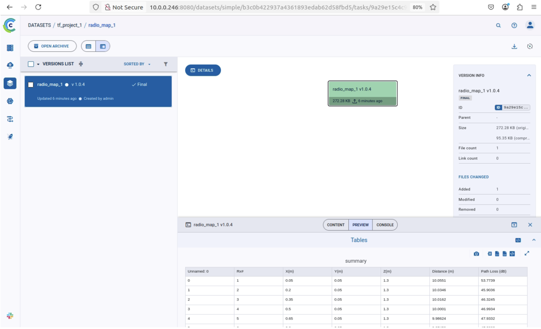
Figure 2: ClearML dashboard showing dataset upload and preview.

Data Preprocessing

Step 8: Clean and filter the dataset (remove invalid rows, drop nulls).

X_actual = df[['X(m)','Y(m)']]
y_actual = df[['Path Loss (dB)']]
df['Path Loss (dB)'] = np.where(df['Path Loss (dB)'] == 250, np.nan, df['Path Loss (dB)'])
df = df.dropna()

Step 9: Split features/labels and scale the data.

x = df[['X(m)', 'Y(m)']].values
y = df[['Path Loss (dB)']].values
x_train, x_test, y_train, y_test = train_test_split(x, y, test_size=0.3, random_state=0)
scaler1 = MinMaxScaler()
x_train = scaler1.fit_transform(x_train)
x_test = scaler1.transform(x_test)
scaler2 = MinMaxScaler()
y_train = scaler2.fit_transform(y_train)
y_test = scaler2.transform(y_test)
X_actual_arr = X_actual.values
X_actual_norm = scaler1.fit_transform(X_actual_arr)

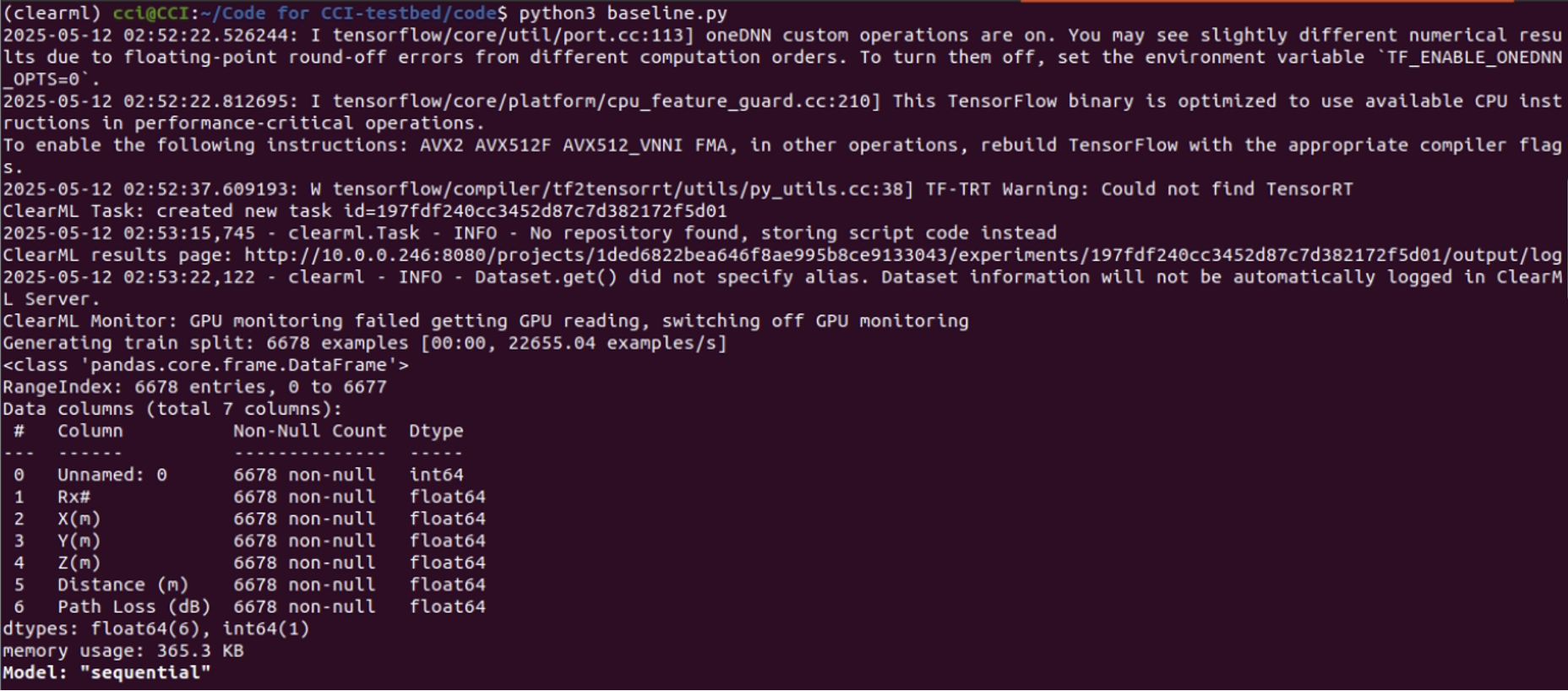
Figure 3: DataFrame info after cleaning and preprocessing.

Model Definition

Step 10: Define a Keras Sequential model for pathloss prediction.

def baseline_model():
    model = Sequential()
    model.add(Dense(64, input_dim=x.shape[1], activation='relu', kernel_initializer='random_normal'))
    # model.add(BatchNormalization())
    # model.add(Dropout(0.2))
    model.add(Dense(32, activation='relu', kernel_initializer='random_normal'))
    # model.add(BatchNormalization())
    # model.add(Dropout(0.2))
    model.add(Dense(16, activation='relu', kernel_initializer='random_normal'))
    model.add(Dense(y.shape[1], activation='relu', kernel_initializer='random_normal'))
    model.compile(optimizer=Adam(learning_rate=0.001), loss='mean_squared_error', metrics=['mean_absolute_error'])
    return model

Model Training with Early Stopping

Step 11: Train the model with early stopping and visualize the training history.

m = baseline_model()
early_stopping = keras.callbacks.EarlyStopping(monitor="val_loss", patience=5, verbose=2)

import time
start_time = time.time()
history = m.fit(x_train, y_train, validation_data=(x_test, y_test), callbacks=[early_stopping], batch_size=16, epochs=120)
end_time = time.time()
duration = end_time - start_time

plot_history(history.history)
task.get_logger().report_matplotlib_figure('Loss curve', "latest model", plt)

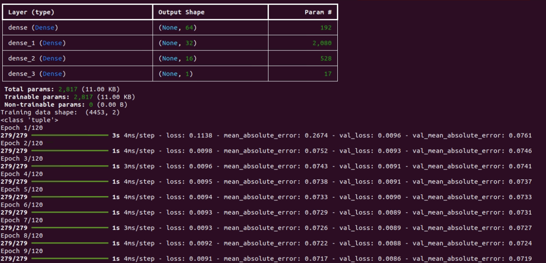
Figure 5: Training and validation loss curve during model training.

Evaluation, Prediction, and Metrics Logging

Step 12: Evaluate the model and make predictions.

y_pred = m.predict(x_test)
print("Test Mean Squared error (MSE):", metrics.mean_squared_error(y_test, y_pred))
print("Test Root mean squared error (RMSE):", np.sqrt(metrics.mean_squared_error(y_test, y_pred)))
print("Test Mean absolute error (MAE):", metrics.mean_absolute_error(y_test, y_pred))
y_pred_flat = y_pred.flatten()
y_test_flat = y_test.flatten()
print("R2 Score Test:", metrics.r2_score(y_test_flat, y_pred_flat))

y_pred_all = m.predict(X_actual_norm)
y_pred_all_inv = scaler2.inverse_transform(y_pred_all)

Step 13: Log metrics and training duration to ClearML.

task.get_logger().report_single_value("Test Mean Squared error (MSE)", metrics.mean_squared_error(y_test, y_pred))
task.get_logger().report_single_value("Test Root mean squared error (RMSE)", np.sqrt(metrics.mean_squared_error(y_test, y_pred)))
task.get_logger().report_single_value("Test Mean absolute error (MAE)", metrics.mean_absolute_error(y_test, y_pred))
task.get_logger().report_single_value("Training time (seconds)", duration)

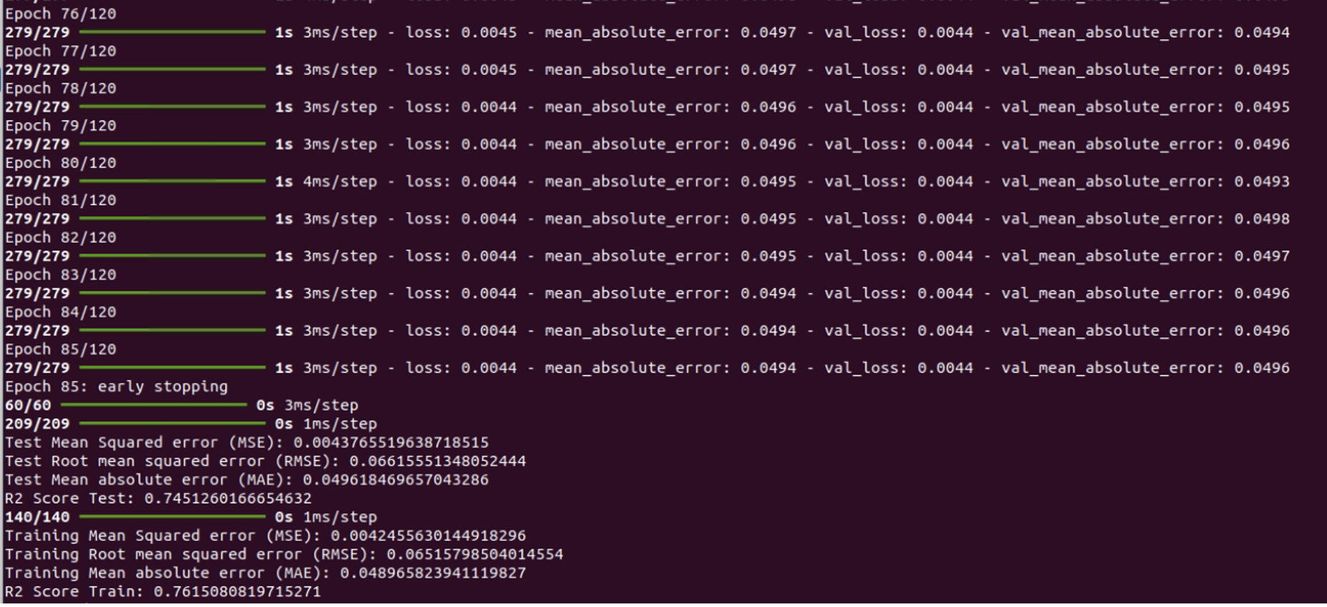
Figure 6: Evaluation metrics and logs in ClearML dashboard.

ClearML Dashboard: Training Results

After completing the model training and evaluation, the ClearML dashboard provides a visual summary of the loss and mean absolute error curves for the completed training task.

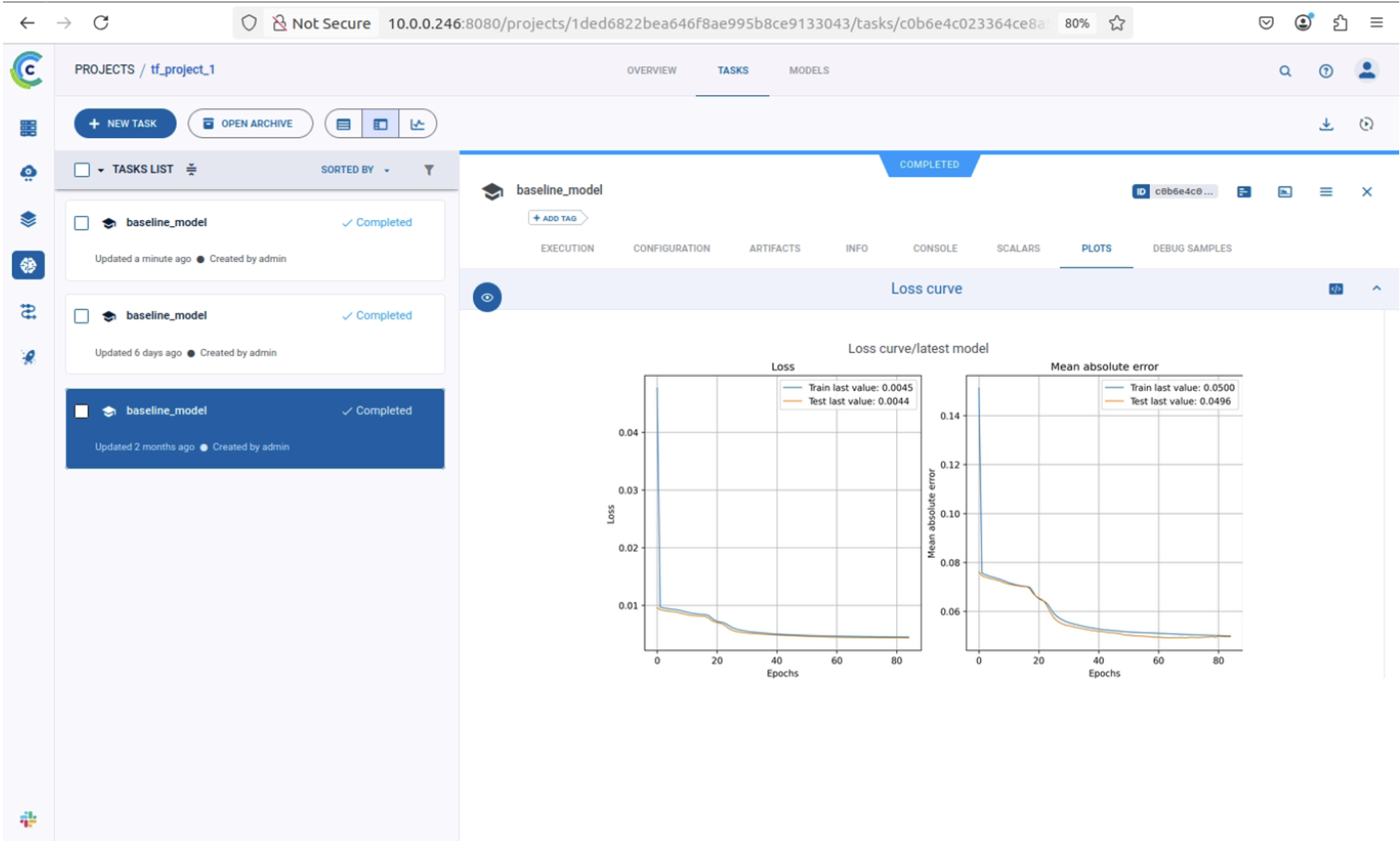
Figure 7: ClearML dashboard showing loss and mean absolute error curves for the completed training task.

Saving the Model

The trained Keras model is saved locally for reuse.

m.save('./serving_model.keras')

Conclusion

This experiment demonstrated how ClearML simplifies end-to-end ML workflow management and experiment tracking. From data preparation to model evaluation, ClearML enabled reproducibility and easy comparison of results for pathloss radio map prediction.

For architectural details and integration, see the ClearML Architecture in the Software Architecture section.

References

[1]

https://clear.ml/docs/latest/docs/

[2]

https://clear.ml/docs/latest/docs/getting_started/ds/ds_first_steps/#auto-log-experiment

[3]

https://clear.ml/docs/latest/docs/clearml_data/clearml_data_sdk